
As a data scientist, you will often be working with tons of data. The form of this data can vary greatly, but pretty often, you can boil it down to tabular structure, that is, in the form of a table like in a spreadsheet.
Suppose you are working in a chemical plant and have a ton of temperature measurements to analyze. Each row is observations and each column is variable.
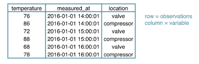
To start working on this data in Python, you will need some kind of rectangular data structure. We have “2D Numpy array”. Well, “2D Numpy array” is an option, but not necessarily the best one. In the above picture, as you can see, there are different data types and Numpy arrays are not great at handing these.
To easily and efficiently handle this data, there is the “Pandas” package. Pandas is a high level data manipulation tool developed by Wes Mckinney, built on the Numpy package.
Compared to Numpy, its more high level, making it very interesting for data scientists all over the world. In pandas, we store the tabular data in an object called a DataFrame.
How can we create DataFrame? Well, there are different ways.
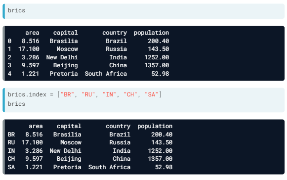
- First of all, you can build it manually, starting from a dictionary. Using the distinctive curly brackets, we can create key value pairs.

As you can see that below, Pandas assigned some automatic row labels, 0 up to 4. To specify them manually, you can set the index attribute of brics to a list with correct labels.
- Well, you will not build the DataFrame manually, Instead, you import data from an external file that contains all this data.

But, the row labels are seen as a column in their own right. To solve this, we will have to tell the read_csv function that the first column contains the row indexes. You can do this by setting the index_col argument, like this.

See you in the next blog !
